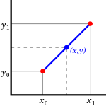
Linear interpolation is all about drawing a line between two points. This example demonstrates the consepts of using linear interpolation with lookup tables to create custom piecewise linear functions.
A line between two points is called a line segment. You can consider one point as the beginning of the segment and the other as the end of the segment. Linear interpolation is about finding any point along this segment.

The goal here is to use linear interpolation to estimate some custom function. Most useful with very complex functions, calibration curves etc.
The first step is to implement simple linear interpolation between two points (x0, y0) and (x1, y1). These two points are the start and end points of a line-segment. Given an x-value, the function outputs the y-value along the segment (the blue (x,y) point illustrated above).
This simple function is so powerful that we are confident enough to define an array of points.. or a sequence of line segments to define our custom function.
Lets take the Sine(x) function from 0 to PI/2 as an example. This is not the most efficient way to calculate sine, but it makes a meaningful example.

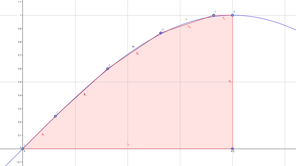
The above graph (red line) is an estimation of the Sine-function using only 6 table points marked with blue dots (A, C, G, H, F, B).
It models one quadrant of the symmetrical cycle of sine.
Points Sin(0) and Sin(PI/2) have accurate values and slopes. Max error is 1% along any segment.
+1% at the points and -1% midway along the segments as they cross the sine-function twice.
Integral of the defined piecewise linear function is 1 (area of the red polygon).
Not bad with only 6 points. It is important to notice that these points can be chosen almost any way we want.
The points do not need to be evenly spaced. Only limitation is that the x-value must increase every step along the function.
With this example piecewise linear function design, we define our data structure and declare the actual sine-table variable.
Now we have a table of (x,y) points. We think of these as a sequence of line-segments.
For a given x-value, we must find the corresponding line-segment and then interpolate to find our y-value.
Because we defined our lookup table to take advantage of the symmetry of the sine function and the periodic nature of the function, we need to write couple of helper functions to give us fully functional interface to calculate Sin(x).
Simple test program.
A graph of the output.

A line between two points is called a line segment. You can consider one point as the beginning of the segment and the other as the end of the segment. Linear interpolation is about finding any point along this segment.
The goal here is to use linear interpolation to estimate some custom function. Most useful with very complex functions, calibration curves etc.
The first step is to implement simple linear interpolation between two points (x0, y0) and (x1, y1). These two points are the start and end points of a line-segment. Given an x-value, the function outputs the y-value along the segment (the blue (x,y) point illustrated above).
C:
/**
* Returns the interpolated y-value.
* Saturates to y0 or y1 if x outside interval [x0, x1].
*/
float interpolate_segment(float x0, float y0, float x1, float y1, float x)
{
    float t;

    if (x <= x0) { return y0; }
    if (x >= x1) { return y1; }

    t =  (x-x0);
    t /= (x1-x0);

    return y0 + t*(y1-y0);
}
/******************************************************************************/
This simple function is so powerful that we are confident enough to define an array of points.. or a sequence of line segments to define our custom function.
Lets take the Sine(x) function from 0 to PI/2 as an example. This is not the most efficient way to calculate sine, but it makes a meaningful example.
The above graph (red line) is an estimation of the Sine-function using only 6 table points marked with blue dots (A, C, G, H, F, B).
It models one quadrant of the symmetrical cycle of sine.
Points Sin(0) and Sin(PI/2) have accurate values and slopes. Max error is 1% along any segment.
+1% at the points and -1% midway along the segments as they cross the sine-function twice.
Integral of the defined piecewise linear function is 1 (area of the red polygon).
Not bad with only 6 points. It is important to notice that these points can be chosen almost any way we want.
The points do not need to be evenly spaced. Only limitation is that the x-value must increase every step along the function.
With this example piecewise linear function design, we define our data structure and declare the actual sine-table variable.
C:
/* Structure definition */
struct table_1d {
    uint8_t x_length;

    float *x_values;
    float *y_values;
};

/* Declare variable using above structure and the function datapoints */
/* These coordinates correspond to the points illustrated in the above graph */
static float sine_x[] = {0.0, 0.24, 0.64, 1.03, 1.43, M_PI_2};
static float sine_y[] = {0.0, 0.24, 0.6,  0.87, 1.00, 1.00};

static struct table_1d sine_table = {
    6,      /* Number of data points */
    sine_x, /* Array of x-coordinates */
    sine_y  /* Array of y-coordinates */
};
Now we have a table of (x,y) points. We think of these as a sequence of line-segments.
For a given x-value, we must find the corresponding line-segment and then interpolate to find our y-value.
C:
float
interpolate_table_1d(struct table_1d *table, float x)
/* 1D Table lookup with interpolation */
{
    uint8_t segment;

    /* Check input bounds and saturate if out-of-bounds */
    if (x > (table->x_values[table->x_length-1])) {
       /* x-value too large, saturate to max y-value */
        return table->y_values[table->x_length-1];
    }
    else if (x < (table->x_values[0])) {
       /* x-value too small, saturate to min y-value */
        return table->y_values[0];
    }

    /* Find the segment that holds x */
    for (segment = 0; segment<(table->x_length-1); segment++)
    {
        if ((table->x_values[segment]   <= x) &&
            (table->x_values[segment+1] >= x))
        {
            /* Found the correct segment */
            /* Interpolate */
            return interpolate_segment(table->x_values[segment],   /* x0 */
                                       table->y_values[segment],   /* y0 */
                                       table->x_values[segment+1], /* x1 */
                                       table->y_values[segment+1], /* y1 */
                                       x);                         /* x  */
        }
    }

    /* Something with the data was wrong if we get here */
    /* Saturate to the max value */
    return table->y_values[table->x_length-1];
}
/******************************************************************************/
Because we defined our lookup table to take advantage of the symmetry of the sine function and the periodic nature of the function, we need to write couple of helper functions to give us fully functional interface to calculate Sin(x).
C:
float
table_sine(float rad)
{
    float y;

    /* Rad should be in the range [0, 2*PI] */
    rad = normalize_radians(rad);

    /* The table is [0, PI/2]. Use Sine-function symmetry with table lookup. */
    if      (rad < (M_PI_2))      { y =  interpolate_table_1d(&sine_table, rad); }
    else if (rad < (M_PI))        { y =  interpolate_table_1d(&sine_table, M_PI-rad); }
    else if (rad < (M_PI+M_PI_2)) { y = -interpolate_table_1d(&sine_table, rad-M_PI); }
    else                          { y = -interpolate_table_1d(&sine_table, (2*M_PI)-rad); }

    return y;
}
/******************************************************************************/

float
normalize_radians(float rad)
/* Normalizes an angle to the range [0, 2*PI[ */
{
    rad = fmod(rad, (2*M_PI));

    if (rad < 0) { return rad+(2*M_PI); }

    return rad;
}
/******************************************************************************/
Simple test program.
C:
/* Test table_sine */
{
    float rad;

    for (rad = -5.0; rad<5.0; rad+=0.05){
        printf("%f\n", table_sine(rad));
        _delay_ms(20);
    }
}
Last edited:
